Mathematical Modeling

Further Mathematics S.S.S 3 Second Term

WEEK 2    

Mathematical Modeling

Performance Objectives

Students should be able to:

1. Explain concept and importance of modeling;
2. Distinguish between dependent and independent variables in modeling
3. State examples of modeling
4. Explain solutions of problems in modeling

Content 

Concept of Mathematical Modeling

Mathematical modeling is a process of applying mathematics to a real life situation. A Model in this context is a simplified, mathematical concept that represents a real life situation.

Mathematical models are developed to help in the understanding of physical phenomena.

The formulation of a model usually involves:

1. making observations;

2. collecting data;

3. carrying out an experiment.

 The observations made or the results of our experiment are then put in mathematical concept that represents a real life situation.

Mathematical models are developed to help in the understanding of physical phenomena.

The formulation of a model usually involves:

1. making observations;

2. collecting data;

3. carrying out an experiment.

The observations made or the results of our experiment are then put in mathematical form together with some assumptions.

This often means representing our observations or experimental results by an equation or set of equations involving some derivatives of one or more unknown functions.

Such equations are called differential equations and these constitute our mathematical model.

Before we proceed further with our model, we need to validate it.

This usually involves solving the corresponding differential equation. It may sometimes be necessary to invent new mathematics to do this. We then interpret the solution and test the predictions of the mathematical model against real-life situations.

In most cases however, it may be necessary to modify the initial model, possibly by removing some of the assumptions made in the formulation of the initial model or applying different mathematical techniques to solve the set of differential equations that constitute the model.

Uses of Mathematical Modeling

Mathematical modeling is widely used in:

1. industry;

2. commerce

3. government;

4. weather forecasting, etc.

Some areas in which mathematical modeling has been successfully used are:

1. population dynamics which includes;

2. predictions of population growths;

3. spread of epidemics such as the HIV/lAIDS virus;

4. financial mathematics, e.g trading in stocks

5. spread of epidemics such as the HIV/ AIDS virus,

6. financial mathematics, e.g trading in stocks;

7. modelling traffic flow;

8. modelling conflicts such as political unrest and wars.

Not only are mathematical models used in the natural sciences such as physics, biology, earth science, meteorology, engineering and computer science especially in artificial intelligence, they are also used in social sciences such as economics, sociology, psychology and political science.

Also, engineers, physicists, statisticians, economists and operations research analysts use mathematical models very extensively.

Examples of Mathematical Models

A simple example of a mathematical model is a geographical projection of a region of the earth onto a small plane area or surface. This model can be used for many purposes such as planning travel.

Another typical mathematical model is predicting the position of a vehicle from its initial position direction and speed of travel using the equation of motion.

A simple model of population growth is the Malthusian growth model. However, a slightly more realistic and largely used population growth model is the logistic function.

In the model of a particle in a potential field for example, a particle is considered as being a point mass which describes a trajectory in space which is modeled by a function whose coordinates in space are given as a function of time.

In physics, movement of rocket model requires, we select and identify relevant aspects of a situation in the real world.

In the model of rational behavior, for a consumer, we assume that a consumer faces a given number of choices of commodities each with a given market price.

Also, the consumer is assumed to have a cardinal utility function in which numerical values are assigned to utilities, depending on the amount of commodities consumed.

Finally, the consumer is also assumed to have a budget which can be used to buy the commodities in such a way as to maximize the utilities.

We see here that the problem of the model of rational behavior becomes the problem of optimization.

Variables in Mathematical Modeling

A mathematical model often describes a system by a set of variables and a set of equations which establish relationships between the variables.

There are six basic groups of variables which form the building blocks of mathematical modeling. These are:

1. decision variables;

2. input variables;

3. state variables;

4. exogenous variables

5.random variables;

6. output variables.

Decision tables are sometimes called independent variables exogenous variables are often referred to as parameters or constants as they are not independent of each other.

The state variables are however dependent on the decision, input random and exogenous variables.

Also the output variables are dependent on the state of the system which is represented by the state variables.

Application of Mathematical Modeling

Mathematical modeling is applied in physical, biological, social and behavioral sciences.

Differential equations are of great importance in these areas since many physical laws and relations appear mathematically in the form of differential equations. We illustrate the essential steps of mathematical modeling by the examples shown below.

Example1

Mathematical model of exponential decay

Scientific experiments show that a radioactive substance decays at a rate proportional to the amount present.

If the initial amount of the radioactive substance is 5 grams, calculate the amount that remains at a later time t.

Solution

 

Step 1

We set up a mathematical model of the physical process which in this case is a differential equation.

We denote by x(t), the amount of substance still present at time t.

From differential calculus,  is the rate of change of decay

From the physical law governing the process of decay Process of decay,    is proportional to x. thus

 ……………………………………………………………….(1)

where k is a definite physical constant whose numerical value is known for various radioactive substance.

It is obvious that as the amount of the radiactive substance is positive and decreases with time, if follows that dxdt is negative and so is k.

We state that the physical process under consideration is described mathematically by an ordinary differential equation of the first order.

Hence, we see that equation (i) is the mathematical model of the physical process

Step 2

The next step is to solve the differential equation.

Given

 = kx …………………………………………………………………(1)

By simple rearrangement we have

 = Kdt ………………………………………………………………..(2)

The process of transforming equation (i) into equation (ii) is called Method of separation of variables.

Integrating both sides of (2) we have

 

  = 

In x = kt + c

X =

=

= Ae^kt( A =

Thus

X = Ae^kt……………………………………………………………………(3)

Equation (iii) above is called the general Solution ofthe differential equation.

 

Step 3

The next step is to find a particular solution.

We observe that the amount of substance x(t) still present at time t will depend on the initial amount of the substance.

This amount is 5 grams at = 0.

We call this the initial condition as it refers to the initial state of the system.

By substituting these initial values i.e x(0) =  5 we have

X(0) = Ae^o

= A

= 5

=> A = 5

If we use this value of A, then the solution (iii) takes the particular form.

X(t) = 5e^kt ………………………………………………………….(4)

 

This particular solution of (1) characterizes the amount of the radioactive substance that remains at any time t ≥ 0.

The physical constant is negative as x(t) decreases as t increases.

Step 4

Validating or checking.

Given that

X = 5e^kt

 = 5e^kt

= k.5e^kt

= kx

Also x(0) = 5e⁰

= 5

Thus x = 5 when t = 0

Hence equation satisfies equation (i) as well as the initial condition.

Example 2

Model of free fall

Experiments show that if a body falls in a vacuum due to the action of gravity, then it experiences a constant acceleration (equal to 9.8m.s^-1, and this is called acceleration due to gravity).

(a) state this law as a differential equation of y(t), the distance fallen as a function of t.

(b) By solving this differential equation show that Y(t) = ½gt²

(c) Assuming the body starts at t = 0 from initial position y = y₀ with initial velocity v = v₀, show that the solution is y(t) = ½gt² + V₀t + y_o

Solution

Given that V(t) is the velocity at any time t, the differential calculus

  is the acceleration at any time t

From experimental results

 

By direct integration with respect to t we have

   

  g 

V = gt + c_1.

V(t) = gt + c₁ ……………………………………………………………………(2)

When t = 0, v(0) = 0

:. 0 = g(0) + c₁

• C₁ = 0……………………………………………………………………..(3)

Thus  V(t) = gt …………………………………………………………….(4)

Now v(t) =  

:.  = gt …………………………………………….…………………………(5)

Integrating both sides of (5) we have

   

  g 

Y = ½gt² + c₂

When t = 0, y(0) = 0

Hence

Y(0) = ½g.(0)² + c₂

• C = 0

Hence y(t0 = ½gt² …………………………..(6)

(C) Given that when t = 0, V = V₀ the we have from equation (2) that:

V₀ = g.o + C₁

• C₁ = V₀……………………………………………(7)

Substituting the value of C₁ in equation (7) into equation (2), WE HAVE

V(t) = gt + V₀ ……………………………………(8)

Since  = v(t), it follows that

 = gt + v₀ ……………………………………………(9)

Integrating both sides of (9) with respect to t we have;

   

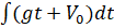
 dy = 12gt² + V₀t + C₂…………………………….(10)

When t = 0, y = y₀

Thus

Y =     g.0² + V₀t + C₂

= y₀

• C₂ = y_o

Hence

Y(t) =gt² + V_0.t + y₂

Example 3

Newton's Law of cooling experiments show that the time rate of change of the temperature T of a body is proportional to the difference between T and the temperature of the surrounding medium. (This is called Newton's law of cooling).

A metal ball is heated to a temperature of 100°C. At time t = 0, it is placed in water which is maintained at a temperature of 30°C. After 3 minutes the temperature of the metal ball reduces to 70°C. Calculate the time at which the temperature of the metal ball reduces to 40^oC.

Solution

Step 1

We set up the mathematical model. In this case, we set up the mathematical formulation of Newton's Law of cooling as:

 = -K(T – 30)…………………………………………(1)

We denote the constant of proportionality by  -k in order to make k >0

Step 2

We find the general solution by solving equation (I) as follows:

 = -K(T – 30)

By separating the variables we have

 = -Kdt …………………………………………….(2)

Integrating both sides of (2) we have

 =  

In (T – 39) = -kt + c

T – 30 = e^{-kt + c}

= e^-kt . e^c

= Ae^-kt

Where A = e^c

Hence T = Ae^-kt + 30 …………………………….(3)

Step 3

We use the initial condition to obtain the particular solution.

T(0) = 100

• 100 = Ae⁰ + 30
• A = 70

Hence T(t) = 70e^-kt + 30 …………………..(4)

Step 4

Making use of further information, we obtain the constant k from the given information

T(3) = 70. We therefore obtain:

T(3) =  70e^-3k + 30

           = 70

Thus 70e^-3k + 30 = 70

70e^-3k = 40

e^-3k = 40/70

      = 4/7

e^3k = 7/4

3k =

K =

= 0.1865.

Substituting the value of k into equation (4),

We have

T(t) = 70e^-0.1865t + 30

It follows that the temperature of 40^oc is reached when T = 40. Thus

70e^-0.1865t + 30 = 40

70e^-0.1865t        = 40 -30

70e^-0.1865t        = 10

e^-0.1865t            = 10/70

e^0.1865t = 7

0.1865t = ln 7

t = ln 7/0.1865

t = 10.43 mins

t ≈.10mins

Hence the temperature of 40^oC is reached after approximately 10 minutes